Langmuir Adsorption Isotherm: Coverage and Linear Plot Numericals
The Langmuir adsorption isotherm is the standard model for gas adsorption on a solid surface, and it appears in the surface chemistry units of IIT-JAM, GATE, CSIR-NET and CUET-PG. The questions are of three kinds: find the fractional coverage, find the pressure needed for a given coverage, and find Vm and K from a table of data by drawing a straight line. This page covers all three.

Assumptions and the equation
Langmuir assumed that the surface has a fixed number of identical sites, each holding one molecule (a monolayer), that adsorbed molecules do not interact, and that adsorption is reversible. Setting the rate of adsorption equal to the rate of desorption gives:
θ = V / Vm
Linear form: P / V = 1 / (K Vm) + P / Vm
- θ is the fraction of surface sites covered (between 0 and 1).
- K is the adsorption equilibrium constant. Its unit is the inverse of the pressure unit (for example kPa−1). A larger K means stronger adsorption.
- P is the pressure of the gas at equilibrium.
- V is the volume of gas adsorbed at pressure P (usually quoted at STP), and Vm is the volume needed to cover the whole surface with one layer.
Two limits are worth remembering. At low pressure (KP << 1), θ ≈ KP, so coverage rises in direct proportion to pressure. At high pressure (KP >> 1), θ → 1 and the surface is saturated; the isotherm flattens. When P = 1/K, exactly half the sites are filled (θ = 0.5).
Example 1: Vm and K from data. Practice data for a gas on a solid at constant temperature:
| P (kPa) | 10 | 20 | 40 | 60 | 80 |
|---|---|---|---|---|---|
| V (cm3) | 10.0 | 16.7 | 25.0 | 30.0 | 33.3 |
| P/V (kPa cm−3) | 1.000 | 1.198 | 1.600 | 2.000 | 2.402 |
Plot P/V against P. The Langmuir equation says the graph is a straight line with slope = 1/Vm and intercept = 1/(K Vm). A least-squares straight-line fit of the five points gives slope = 0.02004 cm−3 and intercept = 0.7982 kPa cm−3.
Vm = 1 / slope = 1 / 0.02004 = 49.9 cm3 (about 50 cm3).
K = slope / intercept = 0.02004 / 0.7982 = 0.0251 kPa−1 (about 0.025 kPa−1).
(The data were built from Vm = 50 cm3 and K = 0.025 kPa−1 and rounded, so the fit recovers them closely. Real data scatter more.)
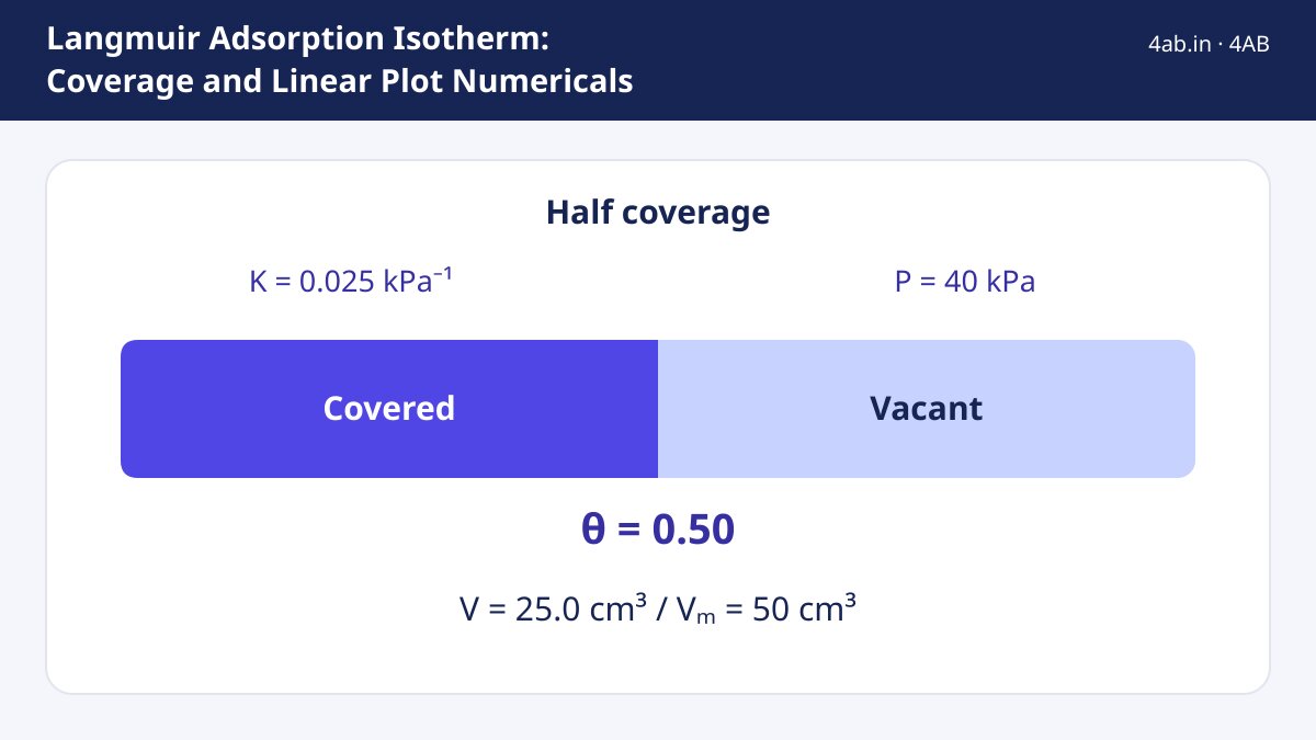
Example 2: coverage at a given pressure. Using K = 0.025 kPa−1 and Vm = 50 cm3, find θ and V at 40 kPa.
KP = 0.025 × 40 = 1.00.
θ = 1.00 / (1 + 1.00) = 0.50.
V = θ Vm = 0.50 × 50 = 25.0 cm3, which agrees with the table in Example 1 (25.0 at 40 kPa). Here P = 1/K = 40 kPa, the half-coverage pressure.
Example 3: pressure needed for high coverage. For K = 0.025 kPa−1, what pressure gives θ = 0.90? Repeat for a stronger adsorbent with K = 0.050 kPa−1 and θ = 0.80.
Rearrange: θ = KP/(1 + KP) gives P = θ / [K (1 − θ)].
First case: P = 0.90 / (0.025 × 0.10) = 0.90 / 0.0025 = 360 kPa.
Second case: the same method for θ = 0.80 and K = 0.050 gives P = 0.80 / (0.050 × 0.20) = 0.80 / 0.010 = 80 kPa.
Check: at K = 0.050 and P = 30 kPa, θ = 1.5 / 2.5 = 0.60. The last 10% of coverage costs a very large increase in pressure, which is why the isotherm flattens.
Example 4: testing the low-pressure limit. For K = 0.025 kPa−1 at P = 1.0 kPa, compare the exact θ with the approximation θ ≈ KP.
Exact: θ = 0.025 / 1.025 = 0.02439.
Approximate: θ ≈ KP = 0.025. The difference is about 2.5%, so the linear approximation is good when KP is about 0.03. At 40 kPa (KP = 1) it would fail badly: it would give θ = 1.0 instead of 0.50.
Langmuir versus Freundlich
The Freundlich isotherm, x/m = k P1/n, is empirical: a plot of log(x/m) against log P is a straight line. It describes moderate pressures well but has no saturation limit. The Langmuir model predicts a limiting amount adsorbed (Vm), so it is the better choice when a flat plateau appears in the data. Also, adsorption is exothermic, so at a higher temperature K becomes smaller and coverage at the same pressure falls.
If a molecule splits into two atoms on adsorption (dissociative adsorption), the form changes to θ = √(KP) / (1 + √(KP)); read the question carefully for this wording.
Common mistakes
- Plotting V against P and calling the line “Langmuir”. The straight-line graph is P/V against P.
- Reading the intercept as 1/Vm. The slope is 1/Vm; the intercept is 1/(K Vm).
- Using the wrong unit for K. If P is in kPa, K is in kPa−1; if P is in bar or atm, K changes numerically.
- Believing θ can exceed 1 at very high pressure. It can only approach 1.
- Applying the Langmuir isotherm to multilayer adsorption. That needs the BET model.
- Forgetting that V and Vm must be given at the same conditions, usually STP.
Exam-relevance table
| Task | Use | Result |
|---|---|---|
| Find coverage | θ = KP/(1 + KP) | value between 0 and 1 |
| Find Vm and K | straight line of P/V vs P | Vm = 1/slope, K = slope/intercept |
| Find pressure for a chosen θ | P = θ / [K(1 − θ)] | pressure in the unit of 1/K |
| Half coverage | P = 1/K | θ = 0.5 |
| Low-pressure behaviour | θ ≈ KP | linear in P |
The exact depth of adsorption questions differs between exams, so check the current official syllabus and past papers for what your exam asks. Drawing a quick table of P/V before fitting the line saves time and catches arithmetic slips.
Fit the straight line P/V against P and read off the slope and intercept without doing the sums by hand.
Open the Linear Regression (Fit y = mx + c) Tool →Step-by-step maths tools for algebra, calculus, matrices and statistics.
More Quantum & structure articles