Standard Addition and Internal Standard Methods in Analysis
A normal calibration curve assumes that the sample behaves like the clean standards. Real samples, such as river water, blood serum or a soil digest, often do not. Other substances in the sample (the matrix) can raise or lower the instrument signal, so the calibration line from pure standards gives a wrong answer. Two methods deal with this problem: the method of standard additions and the internal standard method. Both appear in analytical chemistry sections of IIT-JAM, GATE, CSIR-NET and CUET-PG preparation.

Method of standard additions
Instead of preparing standards in clean water, you add known amounts of the analyte directly to portions of the sample itself. Every portion then has the same matrix, so the matrix effect is the same in all of them and cancels out of the slope. You plot signal against the concentration of analyte added and extend the straight line back to the left until it cuts the x-axis. The distance from the origin to that intercept is the concentration of analyte already present.
Signal = m × Cadded + b
Intercept on the x-axis: Cadded = − b ÷ m
Analyte concentration in the flask, Cflask = b ÷ m
Original sample concentration = Cflask × (final volume ÷ sample volume)
Here m is the slope, and b is the signal at zero addition (the sample alone). The idea is simple: the signal from the sample alone, b, is what the unknown amount produces; dividing by the signal produced per unit added, m, converts it to a concentration.
Conditions for it to work
- The response must be linear over the range used, including the extrapolated part.
- The blank signal must be zero or already subtracted, otherwise the intercept is wrong.
- Each flask must contain the same volume of sample and be made up to the same final volume.
- Extrapolation makes the result less certain than interpolation, so use at least three or four additions.
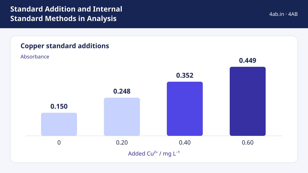
Example 1: copper in a water sample. Four 25.0 mL portions of sample are placed in 50.0 mL flasks. 0, 1.00, 2.00 and 3.00 mL of a 10.0 mg L−1 Cu2+ standard are added, and each flask is made up to 50.0 mL. The absorbance readings are 0.150, 0.248, 0.352 and 0.449.
Step 1: concentration added in each flask. Cadded = (Vstd × 10.0) ÷ 50.0 = 0, 0.20, 0.40, 0.60 mg L−1.
Step 2: least-squares line. n = 4; Σx = 1.20; Σy = 1.199; Σxy = 0.4598; Σx2 = 0.56.
m = (nΣxy − ΣxΣy) ÷ (nΣx2 − (Σx)2) = (4 × 0.4598 − 1.20 × 1.199) ÷ (4 × 0.56 − 1.44) = (1.8392 − 1.4388) ÷ 0.80 = 0.4004 ÷ 0.80 = 0.5005 L mg−1.
b = (Σy − mΣx) ÷ n = (1.199 − 0.5005 × 1.20) ÷ 4 = 0.5984 ÷ 4 = 0.1496.
Step 3: intercept. Cflask = b ÷ m = 0.1496 ÷ 0.5005 = 0.299 mg L−1.
Step 4: undo the dilution. 25.0 mL of sample was made up to 50.0 mL, a factor of 2. Original concentration = 0.299 × 2 = 0.598 mg L−1, about 0.60 mg L−1.
Check: the correlation coefficient of these four points is 0.9999, so the line is very straight. Also m × Cflask = 0.5005 × 0.299 = 0.1496, which is exactly b, the signal of the sample alone.
Internal standard method
Here you add the same fixed amount of a different substance (the internal standard, IS) to every standard and every sample. The IS should behave like the analyte but give a separate signal. You then use the ratio of analyte signal to IS signal. If injection volume, sample loss or instrument drift changes both signals by the same factor, the ratio does not change. This method is common in chromatography.
A = peak area, C = concentration, x = analyte, s = internal standard
For an unknown: Cx = (Ax ÷ As) ÷ F × Cs
Example 2: one-point internal standard. A standard mixture contains 2.00 mg L−1 of analyte X and 5.00 mg L−1 of IS. The peak areas are 3150 (X) and 4200 (IS). A sample is spiked with the same 5.00 mg L−1 IS and gives areas 2800 (X) and 3920 (IS). Find Cx.
F = (3150 ÷ 4200) ÷ (2.00 ÷ 5.00) = 0.7500 ÷ 0.4000 = 1.875.
Sample ratio = 2800 ÷ 3920 = 0.7143.
Cx = (0.7143 ÷ 1.875) × 5.00 = 0.3810 × 5.00 = 1.905 mg L−1 (about 1.91).
Check: the sample ratio 0.7143 is a bit below the standard ratio 0.7500, and the analyte concentration 1.905 is a bit below 2.00. The direction agrees. Also 1.875 × (1.905 ÷ 5.00) = 0.7144, which returns the measured ratio.
Which method when?
| Problem | Best choice |
|---|---|
| Matrix changes the signal (sensitivity differs from clean standards) | Standard additions |
| Injection volume or instrument drift varies from run to run | Internal standard |
| Simple clean samples, many of them | Ordinary external calibration |
| Only a small amount of sample is available | Internal standard is often easier; standard additions needs several portions |
Common mistakes
- Forgetting the dilution factor at the end and quoting the concentration in the flask as the sample concentration.
- Reading the intercept as a positive number. On the x-axis it is negative; the concentration is its size.
- Choosing an internal standard that overlaps with the analyte peak, or that is already present in the sample.
- Using different final volumes in different flasks, which breaks the common-matrix idea.
- Extrapolating far beyond the linear range of the instrument.
Exam relevance
| Exam area | Typical use |
|---|---|
| Analytical chemistry units | Standard addition and internal standard calculations, calibration and detection ideas |
| Instrumental methods | Absorbance, emission and chromatographic quantitation |
Check the current official syllabus and notification of each exam for the topics and depth required.
The standard-addition plot is a straight-line fit of signal against added concentration. Fit the line to your data and read b ÷ m.
Open the Linear Regression Calculator →Step-by-step maths tools for algebra, calculus, matrices and statistics.
More Concepts articles